Cross-Sectional Alpha Factors in Crypto: 2+ Sharpe Ratio Without Overfitting
In the early ’90s, the quant forefathers (Fama and French) introduced their now-canonical factor models: first three, then five, and eventually seven, explaining much of the variation in US equity returns. Today, these models are used to understand what easy-to-replicate risk factors managers are being exposed to. Allocators will want to pay for only the truly unique return sources that can’t be replicated with a couple of lines of SQL.
Crypto markets are currently in the state where many of these “traditional” factors can be still considered alpha, with considerable return potential.
It’s important to note that these cross-sectional factors work without any directional exposure - the regular crypto boom-bust cycle may affect how effective they are, but by design, they have 50-50% long and short exposure at any point in time.
How a Long/Short Factor Portfolio Works — in Brief
Define the universe – e.g., the top 50 digital assets by market cap, updated on a rolling basis to avoid any lookahead bias.
Choose a factor metric – for example, momentum measured as the percentage return over the past n days.
Rank the assets daily based on that metric.
Go long the leaders, short the laggards – take equal-weighted long positions in the top 20% and equal-weighted short positions in the bottom 20%.
This structure isolates the factor exposure while remaining market-neutral.
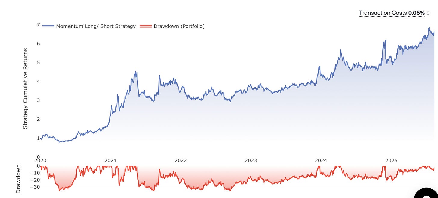
Cross-sectional Momentum
Cross-sectional momentum is a well-documented anomaly: assets that outperform over a given formation period (“winners”) tend to continue outperforming those that underperform (“losers”)—at least in equities.
The same applies to digital assets, with a couple of caveats:
Shorter horizons – In equities, momentum signals often span 6–12 months; in crypto, they’re concentrated over much shorter windows (~30-day formation periods) and decay rapidly, sometimes reversing within months.
Crash-prone behavior – Momentum crashes in crypto are typically triggered by violent reversals in a handful of assets (e.g., short-squeezed losers), rather than broad market shifts.
Large-cap dominance – Most of the returns come from top-40 market-cap coins; smaller tokens suffer from liquidity constraints and higher idiosyncratic risk.
Regime sensitivity – Performance weakens in low-sentiment market regimes.
There’s clear evidence that even the simplest long-only, time-series momentum strategy on Bitcoin have consistently outperforms in risk-adjusted terms - but it works well in the cross-section as well.

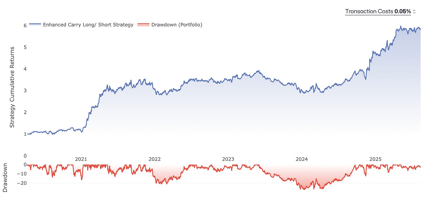
Carry in the cross-section
Unlike momentum, the carry factor traces its roots to commodity markets, where futures often trade at sustained premiums or discounts to spot prices due to factors like storage costs, seasonal patterns, and supply constraints. By expiry, these gaps must close, creating a well-defined arbitrage opportunity.
In crypto, carry is most easily measured via perpetual futures funding rates—periodic payments between traders designed to keep perpetual prices anchored to spot. When perpetuals trade above spot, longs pay shorts; when they trade below, shorts pay longs.
There are two ways to implement carry in this context:
Hard arbitrage – Short assets with high funding rates, buy the same notional exposure in spot, and hedge out any price risk. Profits come directly from the funding payments.
Soft (cross-sectional) carry – Short the assets with the highest funding rates and go long those with the lowest (or most negative), without explicit hedging. Here, returns come from both the funding spread and differences in expected asset performance.
Funding rates vary across exchanges, so we use an open-interest-weighted composite to avoid exchange-specific distortions and better capture the underlying carry signal.

The Caveats
Building crypto-specific, market-neutral, cross-sectional portfolios is far from straightforward. In equities, short availability is a primary constraint; in crypto, the bigger hurdle is survivorship bias—it’s often difficult to source reliable data for delisted or inactive tokens.
Beyond that, most crypto assets—outside of a handful of large-cap names—behave more like penny stocks than mid-cap companies: thinly traded, highly volatile, and frequently subject to pump-and-dump dynamics. Historical testing before ~2020 is of limited use, as the market only reached a comparable level of maturity in the past five years.
Even in this recent period, creating a stable, tradable universe is challenging. We use market cap ranking with additional volume, volatility, and availability filters, with smoothing to limit turnover and avoid overreacting to temporary shifts in liquidity (memecoin spikes).
Another key complication is the dispersion of volatility within the tradable universe. In equities, volatility differences are significant; in crypto, they’re extreme - Bitcoin and the average memecoin might as well be different asset classes. Equal notional long and short positions can still leave the portfolio heavily tilted toward the more volatile side. To address this we apply inverse volatility weighting at the portfolio level so highly volatile tokens get proportionally smaller allocations.
But what’s the alternative to cross-sectional strategies? Potentially overfitting specific signals to individual assets, or abandoning market neutrality entirely.
Achieving Sharpe Ratio of 2+ without Overfitting
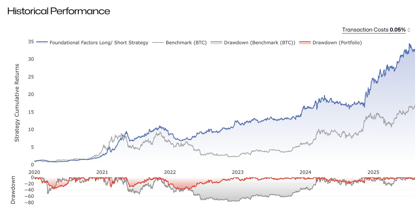
No single factor can consistently forecast returns across all market regimes—it’s an unrealistic expectation. Probably everyone is tired of the mantra “diversification is the only free lunch” - but diversification works particularly well in the context of multi-factor portfolios. The combination doesn’t need to be particularly sophisticated either, even a simple arithmetic average of signals can deliver tangible benefits:
Reduced turnover – When factors disagree, offsetting positions naturally cancel out.
Greatly improved risk-adjusted returns – Uncorrelated return streams smooth the equity curve and raise Sharpe.
When we put these 2 (Momentum + Enhanced Carry) established, well-known factors in a single, portfolio, we get something we call “Foundational” portfolio:
How Far Can This Scale?
Diversification may be the only free lunch, but even free lunches have limits. Once you ensemble more than about six factors, the marginal benefit drops to near zero. We currently track ~20 alpha factors (50 overall) and have found it’s easier to build three orthogonal portfolios with Sharpe ≈ 2.5 than to squeeze a single portfolio up to Sharpe 3.
This breadth puts us in a unique position: we can selectively publish and license some of our proprietary factors without compromising our core edge. You can see their live performance on Unravel, and if you’d like to dig deeper, reach out.
As always, happy to connect on LinkedIn and talk shop!
* The Sharpe Ratio of “Foundational” is actually less than 2, but we track other multi-factor portfolios with considerably higher risk-adjusted returns.


Looks great, thanks for sharing this research! Quick question though - to isolate the factor exposure, wouldn't it make more sense to formulate factor-weighted long/short portfolios (possibly clipping weights to avoid "over dominance'), instead of simple equal weighted?
You mentioned these are market neutral. I don't see how you are neutralizing them.
Just because you do quantiles or rank-weighted doesnt mean they are market neutral.
E.g. for a basic momentum factor, trading quantiles/rank-weight would make it momentum neutral, but not necesarily market neutral, since momentum and market returns can (and good chance are) correlated.